ACCESSIBLE BY clause versus Function Based Indexes
December 14, 2015Oracle introduced the ACCESSIBLE BY clause in 12c to improve the security of subrograms.
Basically the scenario is following:
Let’s create a tax stored function (as hr user) which will be used by the same user in his depts subprogram.
The creator wanted to allow the execution of this function for oe user in it’s total_orders procedure.
CREATE OR REPLACE  FUNCTION TAX(P_AMOUNT IN NUMBER)
RETURN NUMBER
DETERMINISTIC
ACCESSIBLE BY (depts,oe.total_orders)
IS M  NUMBER;
BEGIN
CASE WHEN P_AMOUNT <8000 THEN  M:=0.08; ELSE  M:=0.31;
END CASE;
RETURN P_AMOUNT*M;
END;
/
Function TAX compiled
HR user issued the necessary grant statement:
GRANT EXECUTE ON tax TO oe;
/
Note again, the creator can use this function in his depts procedure, but – for example – in depts2 not!
CREATE OR REPLACE PROCEDURE depts(P_DEPTNO EMPLOYEES.DEPARTMENT_ID%TYPE)
IS
V_max_sal number;
BEGIN
SELECT MAX(salary) INTO v_max_sal
FROM employees
where department_id=p_deptno;
dbms_output.put_line
('The tax value in department('||p_deptno||') is: '||tax(v_max_sal));
END;
/
Procedure DEPTS compiled
However, if hr user wants to create a similar procedure with different name (such as depts2), it will receive an error:
CREATE OR REPLACE PROCEDURE depts2(P_DEPTNO EMPLOYEES.DEPARTMENT_ID%TYPE)
IS
V_max_sal number;
BEGIN
SELECT MAX(salary) INTO v_max_sal
FROM employees
where department_id=p_deptno;
dbms_output.put_line
('The tax value in department('||p_deptno||') is: '||tax(v_max_sal));
END;
/
Error(8,1): PL/SQL: Statement ignored
Error(9,54): PLS-00904: insufficient privilege to access object TAX
This is same for oe user, who wants to use hr’s tax function in total_orders procedure:
CREATE OR REPLACE PROCEDURE total_orders
IS
v_total number;
BEGIN
SELECT sum(order_total) INTO v_total
FROM orders;
dbms_output.put_line('total:'||v_total||' tax of it:'||hr.tax(v_total));
END;
/
Procedure TOTAL_ORDERS compiled
When oe user wants to use hr’s tax function in total_orders2 procedure she or he will receive an Oracle error:
CREATE OR REPLACE PROCEDURE total_orders2
IS
v_total number;
BEGIN
SELECT sum(order_total) INTO v_total
FROM orders;
dbms_output.put_line('total:'||v_total||' tax of it:'||hr.tax(v_total));
END;
/
 PL/SQL: Statement ignored
PLS-00904: insufficient privilege to access object TAX
This information well known, no suprise.
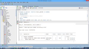
Now hr wants to create a tax_ix function based index for tax function, because he or she wants to improve the performance
for that queries which refer to this function:
CREATE INDEX TAX_IX ON EMPLOYEES(TAX(SALARY));
SQL Error: ORA-06552: PL/SQL: Statement ignored
ORA-06553: PLS-904: insufficient privilege to access object TAX
This behavior is also know from ORACLE-BASE.
(https://oracle-base.com/articles/12c/plsql-white-lists-using-the-accessible-by-clause-12cr1)
What to do?
Let’s modify the definition of the tax function removing the ACCESSIBLE BY clause
CREATE OR REPLACE  FUNCTION TAX(P_AMOUNT IN NUMBER)
RETURN NUMBER
DETERMINISTIC
--ACCESSIBLE BY (depts,oe.total_orders)
IS M  NUMBER;
BEGIN
CASE WHEN P_AMOUNT <8000 THEN  M:=0.08; ELSE  M:=0.31;
END CASE;
RETURN P_AMOUNT*M;
END;
/
Function TAX compiled
Let’s try to create and use the index again:
CREATE INDEX TAX_IX ON EMPLOYEES(TAX(SALARY));
Index TAX_IX created.
We can see that the optimizer used our index in an INDEX RANGE SCAN operation.
Let’s modify our tax function allowing the ACCESSIBLE BY clause:
CREATE OR REPLACE  FUNCTION TAX(P_AMOUNT IN NUMBER)
RETURN NUMBER
DETERMINISTIC
ACCESSIBLE BY (depts,oe.total_orders)
IS M  NUMBER;
BEGIN
CASE WHEN P_AMOUNT <8000 THEN  M:=0.08; ELSE  M:=0.31;
END CASE;
RETURN P_AMOUNT*M;
END;
/
Function TAX compiled
Let’s recompile our depts procedure:
CREATE OR REPLACE PROCEDURE depts(P_DEPTNO EMPLOYEES.DEPARTMENT_ID%TYPE)
IS
V_max_sal number;
BEGIN
SELECT MAX(salary) INTO v_max_sal
FROM employees
where department_id=p_deptno;
dbms_output.put_line
('The tax value in department('||p_deptno||') is: '||tax(v_max_sal));
END;
/
Procedure DEPTS compiled
Now we want to execute the depts procedure as hr:
EXEC depts(90)

Error report -
ORA-06552: PL/SQL: Statement ignored
ORA-06553: PLS-904: insufficient privilege to access object TAX
ORA-06512: at "HR.DEPTS", line 5
It seems to be that hr is underprivileged for executing this function, but
1. The owner of both subrogram is hr.
2. The tax function was allowed for depts procedure to use it.
What is the solution?
According my knowledge I can say
1. Do not create function based index for that function which has
ACCESSIBLE BY clause
2. If you need the function based index, please do not specify ACCESSIBLE BY clause.
Any solution or workaround are appreciated.
Many thanks.
Laszlo
laszlo.czinkoczki@webvalto.hu
How to avoid the persistent state of package’s components?
August 4, 2014Generally the persistent state of package’s component is useful, we don’t want to eliminate it.
Persistency means that the lifetime of package components(variables, cursors,exception definitions, etc.)
start with the instatiation of package and finish with the end of session.
Many developers collect, for example, the necessary exception definitions in a particular package and
later everybody can use them as many times in their session as they want without reloading them into memory.
Sometimes inconvenient, that our session “remembers” the previous state of package components.
Typical scenario when a package is instantiated in one session and later we modify the code of the package in an other session. After this modification in the first session we want to refer to an arbitrary component of the changed component we will get the following error message:
ORA-04068: existing state of packages has been discarded
ORA-04061: existing state of package "HR.CS" has been invalidated
Many times when we want to implement an algoritm with recursion, we need one or more “global variables”.
Let see an example:
Consider the algoritm for the classical “Tower of Hanoi”:
(http://www.mathsisfun.com/games/towerofhanoi.html)
CREATE OR REPLACE PROCEDURE hanoi(first pls_integer,
second pls_integer, n pls_integer)
is
third pls_integer;
BEGIN
IF n=1 THEN
dbms_output.put_line(first||' => '||second);
RETURN;
END IF;
CASE
WHEN  first * second=2 THEN third:=3;
WHEN  first * second=3 THEN third:=2;
WHEN  first * second=6 THEN third:=1;
END CASE;
hanoi(first, third,n-1);
hanoi (first,second,1);
hanoi(third,second,n-1);
END;
/
Whe want to run procedure for 3 level tower then program generates the necessary steps for moving the tower from the first (“1”) position to the second(“2”).
exec hanoi(1,2,3) — we want to move a 3 level tower from the first position to the second
PROCEDURE HANOI compiled
anonymous block completed
1 => 2
1 => 3
2 => 3
1 => 2
3 => 1
3 => 2
1 => 2
Let’s count the number of the steps.
Not surprisingly, the result : 7. (2**3 -1 , where the 3 is the height of the tower).
We want to see step number before printing step instruction.
Not very easy! We can not use a local variabe, we need a “global” variable.
The first attempt could be the following:
Let’s create a package , called hanoi_pkg!
CREATE OR REPLACE PACKAGE hanoi_pkg
is
procedure hanoi(first pls_integer,
second pls_integer, n pls_integer);
END hanoi_pkg;
/
CREATE OR REPLACE PACKAGE BODY hanoi_pkg
IS
i pls_integer:=0;
PROCEDURE hanoi(first pls_integer,
second pls_integer, n pls_integer)
is
third pls_integer;
BEGIN
IF n=1 THEN
i:=i+1;
dbms_output.put_line(i||'. step: '||first||' => '||second);
RETURN;
END IF;
CASE
WHEN  first * second=2 THEN third:=3;
WHEN  first * second=3 THEN third:=2;
WHEN  first * second=6 THEN third:=1;
END CASE;
hanoi(first, third,n-1);
hanoi (first,second,1);
hanoi(third,second,n-1);
END;
END hanoi_pkg;
/
and run the procedure:
exec hanoi_pkg.hanoi(1,2,3)
anonymous block completed
1. step: 1 => 2
2. step: 1 => 3
3. step: 2 => 3
4. step: 1 => 2
5. step: 3 => 1
6. step: 3 => 2
7. step: 1 => 2
The result -seems to be- correct.
Please, run again:
exec hanoi_pkg.hanoi(1,2,3)
anonymous block completed
8. step: 1 => 2
9. step: 1 => 3
10. step: 2 => 3
11. step: 1 => 2
12. step: 3 => 1
13. step: 3 => 2
14. step: 1 => 2
The problem is that our session remembers the latest value of the counter!
The reason is that the components of the package are persistent.
The private variable “i” (see i pls_integer:=0;) is also persistent, even this is a private (not public) variable!
How to solve the problem?
Please use the SERIALLY_REUSABLE pragma ;
The modified package:
CREATE OR REPLACE PACKAGE hanoi_pkg
is
PRAGMA SERIALLY_REUSABLE ;
procedure hanoi(first pls_integer,
second pls_integer, n pls_integer);
END hanoi_pkg;
/
CREATE OR REPLACE PACKAGE BODY hanoi_pkg
IS
i pls_integer:=0;
PRAGMA SERIALLY_REUSABLE ;
PROCEDURE hanoi(first pls_integer,
second pls_integer, n pls_integer)
is
third pls_integer;
BEGIN
IF n=1 THEN
i:=i + 1;
dbms_output.put_line(i||'. step: '||first||' => '||second);
RETURN;
END IF;
CASE
WHEN  first * second=2 THEN third:=3;
WHEN  first * second=3 THEN third:=2;
WHEN  first * second=6 THEN third:=1;
END CASE;
hanoi(first, third,n-1);
hanoi (first,second,1);
hanoi(third,second,n-1);
END;
END hanoi_pkg;
/
Now we test the modification:
exec hanoi_pkg.hanoi(1,2,3)
anonymous block completed
1. step: 1 => 2
2. step: 1 => 3
3. step: 2 => 3
4. step: 1 => 2
5. step: 3 => 1
6. step: 3 => 2
7. step: 1 => 2
Run again – when the package has been instantiated already!)
exec hanoi_pkg.hanoi(1,2,3)
anonymous block completed
1. step: 1 => 2
2. step: 1 => 3
3. step: 2 => 3
4. step: 1 => 2
5. step: 3 => 1
6. step: 3 => 2
7. step: 1 => 2
Finally we can state, that with
PRAGMA SERIALLY_REUSABLE ; statement we removed the instantiated package from the memory.
This can be very useful when we continously develop a package, while other sessions want to use it.
Thanks for visting my site!
My e-mail has changed:
laszlo.czinkoczki@webvalto.hu
but
czinkoczkilaszlo@gmail.com
is still alive.
Temporal validity(history) in Oracle 12c
December 16, 2013In Oracle 11g You can store the previous states of the a table in a Flashback Archive.
Now, starting with Oracle 12c, You can store the old and current states of the rows in the same table.
This is extremely important for dimensonal tables in a Datawarehouse,
because we may want to keep the whole history of a dimension table.
(Consider SCD2 Dimensions)
We can explicitly or implicitly define date/timestamp type columns
that are responsible to store the “lifetime” period of a particular row.
Consider the following scenario:
1. We create a table with invisible(hidden) timestamp columns:
CREATE TABLE my_emp_hidden(
  empno NUMBER,
  last_name VARCHAR2(30),
  PERIOD FOR user_valid_time);
2. Let’s see the generated DDL statement for the table:
SET LONG 10000
SELECT DBMS_METADATA.GET_DDL('TABLE','MY_EMP_HIDDEN','HR') FROM DUAL;
SQL_SCRIPT
-----------
CREATE TABLE "HR"."MY_EMP_HIDDEN"
   (	"EMPNO" NUMBER,
	"LAST_NAME" VARCHAR2(30 BYTE),
	 CONSTRAINT "USER_VALID_TIME9A523" CHECK (USER_VALID_TIME_START < USER_VALID_TIME_END) ENABLE
   ) SEGMENT CREATION IMMEDIATE
  PCTFREE 10 PCTUSED 40 INITRANS 1 MAXTRANS 255
 NOCOMPRESS LOGGING
  STORAGE(INITIAL 65536 NEXT 1048576 MINEXTENTS 1 MAXEXTENTS 2147483645
  PCTINCREASE 0 FREELISTS 1 FREELIST GROUPS 1
  BUFFER_POOL DEFAULT FLASH_CACHE DEFAULT CELL_FLASH_CACHE DEFAULT)
  TABLESPACE "USERS"
  ILM ENABLE LIFECYCLE MANAGEMENT  ;
We can observe a check constraint referring to two (invisible) columns:
USER_VALID_TIME_START and USER_VALID_TIME_END
If you want to see the invisible columns then consider
the following SELECT statement (see Julian Dyke’s blog:
http://www.juliandyke.com/Blog/?p=419)
COL NAME FORMAT A22
COL COL# FORMAT 999
SELECT name,col#,intcol#,segcol#,TO_CHAR (property,'XXXXXXXXXXXX') PROPERTY
FROM sys.col$
WHERE obj# =
(
  SELECT obj# FROM sys.obj$ WHERE name = 'MY_EMP_HIDDEN'
);
NAME                   COL#    INTCOL#    SEGCOL# PROPERTY
---------------------- ---- ---------- ---------- -------------
USER_VALID_TIME_START     0          1          1            20
USER_VALID_TIME_END       0          2          2            20
USER_VALID_TIME           0          3          0         10028
EMPNO                     1          4          3             0
LAST_NAME                 2          5          4             0
The value of COL# is zero for the invisible columns!
3. Now we populate the table with the following 3 rows:
INSERT INTO my_emp_hidden
(empno,last_name,USER_VALID_TIME_START,USER_VALID_TIME_END)
VALUES (100, 'King', to_timestamp('01-Jan-10'), to_timestamp('02-Jun-12'));
INSERT INTO my_emp_hidden
(empno,last_name,USER_VALID_TIME_START,USER_VALID_TIME_END)
VALUES (101, 'Kochhar', to_timestamp('01-Jan-11'), to_timestamp('30-Jun-12'));
INSERT INTO my_emp_hidden
(empno,last_name,USER_VALID_TIME_START,USER_VALID_TIME_END)
VALUES (102, 'De Haan', to_timestamp('01-Jan-12'),NULL);
4. Using the ENABLE_AT_VALID_TIME procedure of DBMS_FLASHBACK_ARCHIVE package
we can see the ALL rows or CURRENT rows only!
EXEC DBMS_FLASHBACK_ARCHIVE.ENABLE_AT_VALID_TIME('ALL')
SELECT * FROM my_emp_hidden;
anonymous block completed
     EMPNO LAST_NAME
---------- ------------------------------
       100 King
       101 Kochhar
       102 De Haan

EXEC DBMS_FLASHBACK_ARCHIVE.ENABLE_AT_VALID_TIME('CURRENT')
SELECT * FROM my_emp_hidden;
anonymous block completed
     EMPNO LAST_NAME
---------- ------------------------------
       102 De Haan
We can see only one row in the second scenario, because we have only one current
(visible) row!
For SQL Tuning experts:
Executions:1 | is_bind_sensitive:N  | is_bind_aware: N | Parsing schema:HR | Disk reads:0 | Consistent gets:183
SQL_ID  445uvm4xj0ar8, child number 0
-------------------------------------
SELECT * FROM my_emp_hidden

Plan hash value: 764633393

-----------------------------------------------------------------------------------
| Id  | Operation         | Name          | Rows  | Bytes | Cost (%CPU)| Time     |
-----------------------------------------------------------------------------------
|   0 | SELECT STATEMENT  |               |       |       |     3 (100)|          |
|*  1 |  TABLE ACCESS FULL| MY_EMP_HIDDEN |     1 |    60 |     3   (0)| 00:00:01 |
-----------------------------------------------------------------------------------

Predicate Information (identified by operation id):
---------------------------------------------------

   1 - filter((("T"."USER_VALID_TIME_START" IS NULL OR
              SYS_EXTRACT_UTC("T"."USER_VALID_TIME_START")<=SYS_EXTRACT_UTC(SYSTIMESTAMP(
              6))) AND ("T"."USER_VALID_TIME_END" IS NULL OR
              SYS_EXTRACT_UTC("T"."USER_VALID_TIME_END")>SYS_EXTRACT_UTC(SYSTIMESTAMP(6))
              )))
5.Valid AS OF PERIOD FOR queries:
-- Returns only King.
SELECT * from my_emp_hidden AS OF PERIOD
FOR user_valid_time TO_TIMESTAMP('01-Jun-10');
    EMPNO LAST_NAME
---------- ------------------------------
       100 King
-- Returns  King and Kochhar.
SELECT * from my_emp_hidden AS OF PERIOD
FOR user_valid_time TO_TIMESTAMP('01-Jun-11');
     EMPNO LAST_NAME
---------- ------------------------------
       100 King
       101 Kochhar

-- Returns Kochhar and De Haan
SELECT * from my_emp_hidden AS OF PERIOD
FOR user_valid_time TO_TIMESTAMP('03-Jun-12');
     EMPNO LAST_NAME
---------- ------------------------------
       101 Kochhar
       102 De Haan
-- Returns all rows
SELECT * from my_emp_hidden VERSIONS PERIOD
FOR user_valid_time
BETWEEN TO_TIMESTAMP('02-jun-11') AND TO_TIMESTAMP('01-May-12');
     EMPNO LAST_NAME
---------- ------------------------------
       100 King
       101 Kochhar
       102 De Haan
-- Returns no rows
SELECT * from my_emp_hidden AS OF PERIOD
FOR user_valid_time TO_TIMESTAMP('01-Jun-09');
no rows selected
If you want to explicitly define the time constraint columns for a table,
consider the documentation
(http://docs.oracle.com/cd/E16655_01/appdev.121/e17620/adfns_design.htm#ADFNS967)
or briefly here:
EXEC DBMS_FLASHBACK_ARCHIVE.ENABLE_AT_VALID_TIME('CURRENT')
CREATE TABLE my_emp(
  empno NUMBER,
  last_name VARCHAR2(30),
  start_time DATE,
  end_time DATE,
PERIOD FOR user_valid_time (start_time, end_time));

INSERT INTO my_emp VALUES (100, 'Ames', '01-Jan-10', '30-Jun-11');
INSERT INTO my_emp VALUES (101, 'Burton', '01-Jan-11', '30-Jun-11');
INSERT INTO my_emp VALUES (102, 'Chen', '01-Jan-12', null);

-- Valid Time Queries --

-- AS OF PERIOD FOR queries:

-- Returns only Ames.
SELECT * from my_emp AS OF PERIOD FOR user_valid_time TO_DATE('01-Jun-10');

-- Returns  Ames and Burton, but not Chen.
SELECT * from my_emp AS OF PERIOD FOR user_valid_time TO_DATE('01-Jun-11');

-- Returns no one.
SELECT * from my_emp AS OF PERIOD FOR user_valid_time TO_DATE( '01-Jul-11');

-- Returns only Chen.
SELECT * from my_emp AS OF PERIOD FOR user_valid_time TO_DATE('01-Feb-12');

-- VERSIONS PERIOD FOR ... BETWEEN queries:

-- Returns only Ames.
SELECT * from my_emp VERSIONS PERIOD FOR user_valid_time BETWEEN
   TO_DATE('01-Jun-10') AND TO_DATE('02-Jun-10');

-- Returns Ames and Burton.
SELECT * from my_emp VERSIONS PERIOD FOR user_valid_time BETWEEN
   TO_DATE('01-Jun-10') AND TO_DATE('01-Mar-11');

-- Returns only Chen.
SELECT * from my_emp VERSIONS PERIOD FOR user_valid_time BETWEEN
   TO_DATE('01-Nov-11') AND TO_DATE('01-Mar-12');

-- Returns no one.
SELECT * from my_emp VERSIONS PERIOD FOR user_valid_time BETWEEN
   TO_DATE('01-Jul-11') AND TO_DATE('01-Sep-11');
no rows selected
SELECT * FROM MY_EMP;
     EMPNO LAST_NAME                      START_TIME END_TIME
---------- ------------------------------ ---------- ---------
       102 Chen                           01-JAN-12
.
This feature is VERY IMPORTANT whenever we want to keep previous versions of the rows
in the same table!
(ps: My e-mail changed! The current is:czinkoczkilaszlo@gmail.com)
Limiting the percentage of ordered rows retrieved in Oracle 12c
July 23, 2013In a previous post I compared two solutions for the same ranking
problem. Now I would like to compare two solutions for the same
percentages report.
The goal of the query: Let's see the first 5% rows of the total
rows according to the salary in descending way.
Let's consider the solution in Oracle 12c, where we can use the
new FETCH {FIRST|NEXT} <pct> PERCENT ROWS clause:
SELECT /*+ GATHER_PLAN_STATISTICS */ employee_id, last_name, salary
FROM employees ORDER BY salary DESC FETCH FIRST 5 PERCENT ROWS
ONLY;
EMPLOYEE_ID LAST_NAME SALARY
----------- ------------ --------
100 King 24000
101 Kochhar 17000
102 De Haan 17000
145 Russell 14000
146 Partners 13500
201 Hartstein 13000
6 rows selected
One of the possible traditional solution uses
the cumulative distribution (CUME_DIST) analytic function.
SELECT /*+ GATHER_PLAN_STATISTICS */ E.*
FROM
(SELECT employee_id, last_name, salary,
CUME_DIST() OVER( ORDER BY Salary DESC) cum_dist
FROM employees ORDER BY salarY DESC) E
WHERE E.CUM_DIST<=0.05;
EMPLOYEE_ID LAST_NAME SALARY CUM_DIST
----------- --------- ---------- -------------
100 King 24000 0.009345794393
101 Kochhar 17000 0.02803738318
102 De Haan 17000 0.02803738318
145 Russell 14000 0.03738317757
146 Partners 13500 0.04672897196
Let's consider the execution plan for that query which
uses the new FETCH {FIRST|NEXT} <pct> PERCENT ROWS clause:
Executions:1 | is_bind_sensitive:N | is_bind_aware: N | Parsing schema:HR | Disk reads:0 | Consistent gets:1555
SQL_ID 1jnwttv1rt22u, child number 0
-------------------------------------
SELECT /*+ GATHER_PLAN_STATISTICS */ employee_id, last_name, salary
FROM employees ORDER BY salary DESC FETCH FIRST 5 PERCENT ROWS ONLY
Plan hash value: 720055818
---------------------------------------------------------------------------------
| Id | Operation | Name | Rows | Bytes | Cost (%CPU)| Time |
---------------------------------------------------------------------------------
| 0 | SELECT STATEMENT | | | | 3 (100)| |
|* 1 | VIEW | | 107 | 8453 | 3 (0)| 00:00:01 |
| 2 | WINDOW SORT | | 107 | 1712 | 3 (0)| 00:00:01 |
| 3 | TABLE ACCESS FULL| EMPLOYEES | 107 | 1712 | 3 (0)| 00:00:01 |
---------------------------------------------------------------------------------
Predicate Information (identified by operation id):
---------------------------------------------------
1 - filter("from$_subquery$_002"."rowlimit_$$_rownumber"<=CEIL("from$_
subquery$_002"."rowlimit_$$_total"*5/100))
Operation_id:1 last ouput rows:6 Query block name: SEL$1
Operation_id:2 last ouput rows:107 Query block name: SEL$1
Operation_id:3 last ouput rows:107 Query block name: SEL$1
====================================================================================================
Now we examine the execution plan of the query that uses the CUME_DIST analytic function:
Executions:1 | is_bind_sensitive:N | is_bind_aware: N | Parsing schema:HR | Disk reads:0 | Consistent gets:7
SQL_ID 0u2b7mdnfy5nh, child number 0
-------------------------------------
SELECT /*+ GATHER_PLAN_STATISTICS */ E.* FROM (SELECT employee_id,
last_name, salary, CUME_DIST() OVER( ORDER BY Salary DESC) cum_dist
FROM employees ORDER BY salarY DESC) E WHERE E.CUM_DIST<=0.05
Plan hash value: 720055818
---------------------------------------------------------------------------------
| Id | Operation | Name | Rows | Bytes | Cost (%CPU)| Time |
---------------------------------------------------------------------------------
| 0 | SELECT STATEMENT | | | | 3 (100)| |
|* 1 | VIEW | | 107 | 5671 | 3 (0)| 00:00:01 |
| 2 | WINDOW SORT | | 107 | 1712 | 3 (0)| 00:00:01 |
| 3 | TABLE ACCESS FULL| EMPLOYEES | 107 | 1712 | 3 (0)| 00:00:01 |
---------------------------------------------------------------------------------
Predicate Information (identified by operation id):
---------------------------------------------------
1 - filter("E"."CUM_DIST"<=.05)
Operation_id:1 last ouput rows:5 Query block name: SEL$2
Operation_id:2 last ouput rows:107 Query block name: SEL$2
Operation_id:3 last ouput rows:107 Query block name: SEL$2
====================================================================================================
We can observe that BOTH queries use the SAME EXECUTION plan,
but with different number of consistent gets (1551 versus 7!).
Other metrics are same.
I created a greater table:
CREATE TABLE big_emp(empno,last_name,first_name,salary)
AS
SELECT ROWNUM,E.last_name||ROWNUM,E.first_name||ROWNUM,E.salary
FROM employees E,employees D,employees F;
SELECT COUNTt(*) FROM big_emp;
COUNT(*)
----------
1225043
I executed the following queries:
SELECT /*+ GATHER_PLAN_STATISTICS */ *
FROM big_emp ORDER BY salary DESC FETCH FIRST 1 PERCENT ROWS
ONLY;
SELECT /*+ GATHER_PLAN_STATISTICS */ E.*
FROM
(SELECT b.*,
CUME_DIST() OVER( ORDER BY Salary DESC) cum_dist
FROM big_emp b ORDER BY salarY DESC) E
WHERE E.CUM_DIST<=0.01;
Of course, I got the same execution plan.
But the were no big difference between the number of consistent gets.
Executions:1 | is_bind_sensitive:N | is_bind_aware: N | Parsing schema:HR | Disk reads:0 | Consistent gets:6693
SQL_ID 5cv1yxs3aht9g, child number 0
-------------------------------------
SELECT /*+ GATHER_PLAN_STATISTICS */ E.* FROM (SELECT b.*, CUME_DIST()
OVER( ORDER BY Salary DESC) cum_dist FROM big_emp b ORDER BY salarY
DESC) E WHERE E.CUM_DIST<=0.01
Plan hash value: 1432758025
Executions:1 | is_bind_sensitive:N | is_bind_aware: N | Parsing schema:HR | Disk reads:6684 | Consistent gets:8059
SQL_ID gg7n3x4px3tak, child number 0
-------------------------------------
SELECT /*+ GATHER_PLAN_STATISTICS */ * FROM big_emp ORDER BY salary
DESC FETCH FIRST 1 PERCENT ROWS ONLY
Plan hash value: 1432758025
The number of consistent gets were
(6693- for traditional versus 8059 - new for feature)
As I saw we can use both solutions,but the FETCH clause
is more readable and user-friend.
Restricted access to PL/SQL subprograms in Oracle 12c
July 10, 2013Prior to Oracle 12c everyone can refer to a subprogram (helper program) in an other PL/SQL program unit if that user has execute privilege for the helper object or owns it.
Now, in Oracle 12c the creator of the helper can determine that
which program units can refer to it, even the other users have execute privilege for the helper objects or they have the EXECUTE ANY PRIVILEGE system privilege.
Even the the owner of the helper object is same as the PL/SQL
subprogram’s owner, but if the dependent object is not entitled to use
the helper subprogram it can not refer to helper PL/SQL subprogram.
The new feature is that the helper PL/SQL subprogram can have
an ACCESSIBLE BY (subprogram1,subprogram2, …) clause where the creator can provide the access to the subprograms listed after the ACCESSIBLE BY keywords.
In the following example HR user who created the tax function provided access of the tax function to the depts procedure (owned by HR) and to depts2 owned by CZINK user.
Note that HR issued the suitable object privilege to czink.
Let’s see the definition of the tax function and the GRANT statement:
CREATE OR REPLACE FUNCTION tax(BASE NUMBER)
RETURN NUMBER
ACCESSIBLE BY (depts,czink.depts2)
IS
S NUMBER;
BEGIN
IF BASE<4000 THEN
  S:= 0.10;
ELSIF BASE<20000 THEN
  S:=0.25;
ELSE
  S:=0.3;
END IF;
RETURN BASE*S;
END;
/
GRANT EXECUTE ON tax TO czink;
Now HR user created a procedure called depts and executed it:
CREATE OR REPLACE
PROCEDURE depts(p_deptno  employees.department_id%TYPE)
AUTHID CURRENT_USER
IS
CURSOR c_emp(c_deptno employees.department_id%TYPE) IS
SELECT e.*, 12*salary*(1+NVL(commission_pct,0)) ANN_SAL
FROM employees e WHERE department_id=c_deptno;
manager employees.last_name%TYPE;
BEGIN
FOR r  IN c_emp(p_deptno) LOOP
    IF r.manager_id IS NOT NULL THEN
     SELECT last_name INTO MANAGER FROM employees
     WHERE employee_id=r.manager_id;
   ELSE
    manager:='No Manager';
   END IF;
   DBMS_OUTPUT.PUT_LINE(c_emp%ROWCOUNT||'. name:='||r.last_name||' salary:'||r.salary||
   ' tax:'|| tax(r.salary) ||  ' Manager:'||manager||' '||r.manager_id||' Annual Salary:'||r.ann_sal);
END LOOP;
EXCEPTION
 WHEN OTHERS THEN
dbms_output.put_line('The error:'||DBMS_UTILITY.FORMAT_ERROR_STACK );
END;
/
exec depts(90)
anonymous block completed
1. name:=King salary:24000 tax:7200 Manager:No Manager  Annual Salary:288000
2. name:=Kochhar salary:17000 tax:4250 Manager:King 100 Annual Salary:204000
3. name:=De Haan salary:17000 tax:4250 Manager:King 100 Annual Salary:204000
However if HR wants to create a depts2 procedure with the
following code, Oracle produces an error message, because the depts2 procedure WAS NOT ENTITLED to refer to the tax function:
CREATE OR REPLACE
PROCEDURE depts2(p_deptno  employees.department_id%TYPE)
AUTHID CURRENT_USER
IS
CURSOR c_emp(c_deptno employees.department_id%TYPE) IS
SELECT e.*, 12*salary*(1+NVL(commission_pct,0)) ANN_SAL
FROM employees e WHERE department_id=c_deptno;
manager employees.last_name%TYPE;
BEGIN
FOR r  IN c_emp(p_deptno) LOOP
    IF r.manager_id IS NOT NULL THEN
     SELECT last_name INTO MANAGER FROM employees
     WHERE employee_id=r.manager_id;
   ELSE
    manager:='No Manager';
   END IF;
   DBMS_OUTPUT.PUT_LINE(c_emp%ROWCOUNT||'. name:='||r.last_name||' salary:'||r.salary||
   ' tax:'|| tax(r.salary) ||  ' Manager:'||manager||' '||r.manager_id||' Annual Salary:'||r.ann_sal);
END LOOP;
EXCEPTION
 WHEN OTHERS THEN
dbms_output.put_line('The error:'||DBMS_UTILITY.FORMAT_ERROR_STACK );
END;
/
Error(17,14): PLS-00904: insufficient privilege to access object TAX
Now CZINK user wants to create and execute a depts2 procedure
referring to the tax function owned by HR:
(Supposed that CZINK user has it’s own employees table)
CREATE OR REPLACE
PROCEDURE depts2(p_deptno  employees.department_id%TYPE)
AUTHID CURRENT_USER
IS
CURSOR c_emp(c_deptno employees.department_id%TYPE) IS
SELECT e.*, 12*salary*(1+NVL(commission_pct,0)) ANN_SAL
FROM employees e WHERE department_id=c_deptno;
manager employees.last_name%TYPE;
BEGIN
FOR r  IN c_emp(p_deptno) LOOP
IF r.manager_id IS NOT NULL THEN
SELECT last_name INTO MANAGER FROM employees
WHERE employee_id=r.manager_id;
ELSE
manager:='No Manager';
END IF;
DBMS_OUTPUT.PUT_LINE(c_emp%ROWCOUNT||'. name:='||r.last_name||' salary:'||r.salary||
' tax:'|| HR.tax(r.salary) ||  ' Manager:'||manager||' '||r.manager_id||' Annual Salary:'||r.ann_sal);
END LOOP;
EXCEPTION
WHEN OTHERS THEN
dbms_output.put_line('The error:'||DBMS_UTILITY.FORMAT_ERROR_STACK );
END;
/
exec depts2(90)
anonymous block completed
1. name:=King salary:24000 tax:7200 Manager:No Manager  Annual Salary:288000
2. name:=Kochhar salary:17000 tax:4250 Manager:King 100 Annual Salary:204000
3. name:=De Haan salary:17000 tax:4250 Manager:King 100 Annual Salary:204000
Of course, if CZINK user created a procedure
(referring to HR’s tax function) with different name than depts2
then CZINK user would get the same error message.
(The DBA role was assigned to the CZINK user in my example)
Comment and benefits of using the ACCESSIBLE BY clause:
1. You can provide access to a helper PL/SQL programs only for those
PL/SQL subprograms which are really need to refer to them.
2. The restriction made for PL/SQL subprograms not for users.
3. Even if a user has a DBA role or “just” the
EXECUTE ANY PROCEDURE the user won’t be able to use the helper
PL/SQL subprogram, unless it(the helper program) allows
to access directly to the invoker program.
4. You can specify the ACCESSIBLE BY clause on package level
(not for individual members), like this:
CREATE OR REPLACE PACKAGE taxes ACCESSIBLE BY (depts,czink.depts2)
IS
FUNCTION tax1(BASE NUMBER) RETURN NUMBER;
FUNCTION tax2(BASE NUMBER) RETURN NUMBER;
END taxes;
/
CREATE OR REPLACE PACKAGE BODY taxes
IS
FUNCTION tax1(BASE NUMBER) RETURN NUMBER
IS
S NUMBER;
BEGIN
IF    BASE<4000 THEN   S:= 0.10;
ELSIF BASE<20000 THEN   S:=0.25;
ELSE  S:=0.3;
END IF;
RETURN BASE*S;
END tax1;
FUNCTION tax2(BASE NUMBER) RETURN NUMBER
IS
S NUMBER;
BEGIN
IF BASE<4000 THEN   S:= 0.10;
ELSE   S:=0.3;
END IF;
RETURN BASE*S;
END tax2;
END taxes;
/
Work with WITH option in Oracle 12c!
July 9, 2013Starting Oracle 9.0 – according to SQL 1999 standard – Oracle introduced the WITH option which can be considered
as the extension of the inline views.
Let’s see an “old” example:
WITH
dept_costs  AS
(SELECT department_name, SUM(salary) as dept_total
FROM employees, departments
WHERE employees.department_id =
departments.department_id
GROUP BY department_name),
avg_cost  AS
(SELECT SUM(dept_total)/COUNT(*) as dept_avg
FROM   dept_costs)
SELECT * FROM dept_costs
WHERE dept_total >
(SELECT dept_avg FROM  avg_cost)
ORDER BY department_name;
(The origin of this statement is Oracle course,titled:
Oracle Database: SQL Fundamentals I
Volume II • Student Guide).
In Oracle 12c we have new enhancements for this kind of SQL statement:
We can define “in-line” functions or procedures after the WITH clause.
In the following example we are looking for those departments, where
total salary of the department is greater than the maximum of the average of the total salaries:
WITH
FUNCTION tax(p_amount IN NUMBER)
RETURN NUMBER
IS
m  NUMBER;
BEGIN
IF p_amount <8000 THEN
m:=0.08;
ELSIF p_amount <18000 THEN
m:=0.25;
ELSE
m:=0.3;
END IF;
RETURN p_amount * m;
END;
emp_costs  AS (
SELECT d.department_name dept_name,e.last_name, e.salary AS salary,
tax(e.salary) AS tax_amount
FROM   employees e JOIN departments d
ON     e.department_id = d.department_id),
dept_costs    AS (
SELECT dept_name, SUM(salary) AS dept_sal,SUM(tax_amount) tax_sum,
AVG(salary) avg_sal
FROM   emp_costs GROUP BY dept_name)
SELECT * FROM   dept_costs
WHERE  dept_sal > (SELECT MAX(avg_sal) FROM dept_costs)
ORDER BY dept_name;
/
The result is:
DEPT_NAME             DEPT_SAL    TAX_SUM    AVG_SAL
------------------------------ ---------- ---------- ----------
Accounting               20308       5077      10154
Executive                58000      15700 19333.3333
Finance                  51608       9094 8601.33333
IT                       28800       3834       5760
Purchasing               24900       3862       4150
Sales                   304500      62083 8955.88235
Shipping                156400      15266 3475.55556

7 rows selected.
The execution plan is the following ( not very simple!):
Plan hash value: 38700341

-------------------------------------------------------------------------------------------------------------
| Id  | Operation                       | Name                      | Rows  | Bytes | Cost (%CPU)| Time     |
-------------------------------------------------------------------------------------------------------------
|   0 | SELECT STATEMENT                |                           |       |       |     7 (100)|          |
|   1 |  TEMP TABLE TRANSFORMATION      |                           |       |       |            |          |
|   2 |   LOAD AS SELECT                |                           |       |       |            |          |
|   3 |    HASH GROUP BY                |                           |    27 |   621 |     3   (0)| 00:00:01 |
|   4 |     NESTED LOOPS                |                           |       |       |            |          |
|   5 |      NESTED LOOPS               |                           |   106 |  2438 |     3   (0)| 00:00:01 |
|   6 |       TABLE ACCESS FULL         | EMPLOYEES                 |   107 |   749 |     3   (0)| 00:00:01 |
|*  7 |       INDEX UNIQUE SCAN         | DEPT_ID_PK                |     1 |       |     0   (0)|          |
|   8 |      TABLE ACCESS BY INDEX ROWID| DEPARTMENTS               |     1 |    16 |     0   (0)|          |
|   9 |   SORT ORDER BY                 |                           |    27 |  1512 |     4   (0)| 00:00:01 |
|* 10 |    VIEW                         |                           |    27 |  1512 |     2   (0)| 00:00:01 |
|  11 |     TABLE ACCESS FULL           | SYS_TEMP_0FD9D6694_1CABAF |    27 |   621 |     2   (0)| 00:00:01 |
|  12 |     SORT AGGREGATE              |                           |     1 |    13 |            |          |
|  13 |      VIEW                       |                           |    27 |   351 |     2   (0)| 00:00:01 |
|  14 |       TABLE ACCESS FULL         | SYS_TEMP_0FD9D6694_1CABAF |    27 |   621 |     2   (0)| 00:00:01 |
-------------------------------------------------------------------------------------------------------------

Predicate Information (identified by operation id):
---------------------------------------------------

7 - access("E"."DEPARTMENT_ID"="D"."DEPARTMENT_ID")
10 - filter("DEPT_SAL">)

====================================================================================================</pre>
We can use the WITH option with plsql_declarations clause
in DML statements as well.
Let’s consider the following example where we want to compute the
tax amount of the salaries and modify the tax_amount column,
but we DON’T WANT TO USE the stored tax function if exists at all!
First we create a copy of the employees table and modify the
structure with a new column
CREATE TABLE newmp AS SELECT * FROM employees;
ALTER TABLE newemp ADD tax_amount NUMBER(10,2);
Now we modify the content of the tax_amount column
(which is originally empty) with each employee’s tax amount:
UPDATE     /*+ WITH_PLSQL */ newemp E
SET tax_amount=(WITH FUNCTION TAX(P_AMOUNT IN NUMBER)
RETURN NUMBER
IS
M  NUMBER;
BEGIN
IF P_AMOUNT <8000 THEN
M:=0.08;
ELSIF P_AMOUNT <18000 THEN
M:=0.25;
ELSE
M:=0.3;
END IF;
RETURN P_AMOUNT*M;
END;
SELECT tax(salary) FROM employees m
WHERE m.employee_id=e.employee_id)
/
Observe that the WITH statement has a special hint.
The WITH_PLSQL hint only enables you to specify
the WITH plsql_declarations clause within the statement.
It is not an optimizer hint.(see Oracle 12c documentation)
Let’s check the result (only the first 10 rows are displayed):
SELECT *
FROM
(SELECT  last_name,salary,tax_amount from newemp
ORDER BY  salary DESC)
WHERE ROWNUM<=10;

LAST_NAME                          SALARY TAX_AMOUNT
-------------------------      ---------- ----------
King                                24000       7200
Kochhar                             17000       4250
De Haan                             17000       4250
Russell                             14000       3500
Partners                            13500       3375
Hartstein                           13000       3250
Greenberg                           12008       3002
Higgins                             12008       3002
Errazuriz                           12000       3000
Ozer                                11500       2875

10 rows selected.
The execution plan for the UPDATE is the following(simpler!)
Executions:1 | is_bind_sensitive:N  | is_bind_aware: N | Parsing schema:HR | Disk reads:0 | Consistent gets:505
SQL_ID  6s126hzr93g2d, child number 0
-------------------------------------
UPDATE  /*+ WITH_PLSQL */ newemp E SET tax_amount=(WITH FUNCTION
TAX(P_AMOUNT IN NUMBER) RETURN NUMBER IS M  NUMBER; BEGIN IF P_AMOUNT
<8000 THEN M:=0.08; ELSIF P_AMOUNT <18000 THEN M:=0.25; ELSE M:=0.3;
END IF; RETURN P_AMOUNT*M; END; SELECT tax(salary) FROM employees m
WHERE m.employee_id=e.employee_id)

Plan hash value: 759157450

----------------------------------------------------------------------------------------------
| Id  | Operation                    | Name          | Rows  | Bytes | Cost (%CPU)| Time     |
----------------------------------------------------------------------------------------------
|   0 | UPDATE STATEMENT             |               |       |       |   217 (100)|          |
|   1 |  UPDATE                      | NEWEMP        |       |       |            |          |
|   2 |   TABLE ACCESS FULL          | NEWEMP        |   107 |  1819 |     3   (0)| 00:00:01 |
|   3 |   TABLE ACCESS BY INDEX ROWID| EMPLOYEES     |     1 |     8 |     1   (0)| 00:00:01 |
|*  4 |    INDEX UNIQUE SCAN         | EMP_EMP_ID_PK |     1 |       |     0   (0)|          |
----------------------------------------------------------------------------------------------

Predicate Information (identified by operation id):
---------------------------------------------------

4 - access("M"."EMPLOYEE_ID"=:B1)

====================================================================================================
The greatest benefit of using PL/SQL functions or procedures that we
can use our (not stored) subprograms in queries without writing
procedural code.
Limiting the number of ordered rows retrieved in Oracle 12c
July 9, 2013Starting with Oracle 12c You can limit the ordered result set of a query with FETCH clause after the ORDER BY clause.
Earlier You had to use analytic function for solving this problem.
Now -with the new syntax- you can implement it with easier syntax,
but the execution plan is SAME, as you will see it.
Let’s consider the following ranking problem:
We would like to see the first “n” well paid people from employees
table using the traditional RANK analytic function:
SELECT  /*+ GATHER_PLAN_STATISTICS */  t.*
FROM(SELECT employee_id,last_name,salary,
RANK()
 OVER( ORDER BY  salary desc) rank from employees) t
WHERE t.rank<=2
100 King               24000         1
101 Kochhar            17000         2
102 De Haan            17000         2
As You could see that the server fetched 3 rows because
the last 2 employee have the same salaries.
Now consider the new FETCH opertor with FIRST/NEXT
(they are same!):
SELECT /*+ GATHER_PLAN_STATISTICS */  employee_id, last_name, salary
FROM employees
ORDER BY salary DESC
FETCH NEXT 5 ROWS ONLY ;
100 King                  24000
101 Kochhar               17000
102 De Haan               17000
145 Russell               14000
146 Partners              13500
Nice feature is the OFFSET clause, which enables us to fetch next “n”rows after “m” rows:
SELECT /*+ GATHER_PLAN_STATISTICS */  employee_id, last_name, salary
FROM employees
ORDER BY salary DESC OFFSET 5 ROWS
FETCH NEXT 5 ROWS ONLY  ;
201 Hartstein             13000
108 Greenberg             12008
205 Higgins               12008
147 Errazuriz             12000
168 Ozer                  11500
Now let’s see the execution plans! You will see – even the number of the rows are different – the SAME EXECUTION PLAN was used
by the optimizer, first for the RANK function:
Executions:1 | is_bind_sensitive:N  | is_bind_aware: N | Parsing schema:HR | Disk reads:0 | Consistent gets:275
SQL_ID  fb0u8y9g33ykp, child number 0
-------------------------------------
SELECT  /*+ GATHER_PLAN_STATISTICS */  t.* FROM (SELECT
employee_id,last_name,salary,  RANK() OVER( ORDER BY  salary desc) rank
from employees) t  WHERE t.rank<=2

Plan hash value: 2698234872

--------------------------------------------------------------------------------------
| Id  | Operation                | Name      | Rows  | Bytes | Cost (%CPU)| Time     |
--------------------------------------------------------------------------------------
|   0 | SELECT STATEMENT         |           |       |       |     3 (100)|          |
|*  1 |  VIEW                    |           |   107 |  5671 |     3   (0)| 00:00:01 |
|*  2 |   WINDOW SORT PUSHED RANK|           |   107 |  1712 |     3   (0)| 00:00:01 |
|   3 |    TABLE ACCESS FULL     | EMPLOYEES |   107 |  1712 |     3   (0)| 00:00:01 |
--------------------------------------------------------------------------------------

Predicate Information (identified by operation id):
---------------------------------------------------

1 - filter("T"."RANK"<=2)
2 - filter(RANK() OVER ( ORDER BY INTERNAL_FUNCTION("SALARY") DESC )<=2)

Operation_id:1 last ouput rows:3 Query block name: SEL$2
Operation_id:2 last ouput rows:3 Query block name: SEL$2
Operation_id:3 last ouput rows:107 Query block name: SEL$2
====================================================================================================
Let’s consider the execution plan for the first FETCH operator:
(without OFFSET option)
Executions:1 | is_bind_sensitive:N  | is_bind_aware: N | Parsing schema:HR | Disk reads:0 | Consistent gets:7
SQL_ID  3hp4dwmhuvp7b, child number 0
-------------------------------------
SELECT /*+ GATHER_PLAN_STATISTICS */  employee_id, last_name, salary
FROM employees  ORDER BY salary DESC FETCH NEXT 5 ROWS ONLY

Plan hash value: 2698234872

--------------------------------------------------------------------------------------
| Id  | Operation                | Name      | Rows  | Bytes | Cost (%CPU)| Time     |
--------------------------------------------------------------------------------------
|   0 | SELECT STATEMENT         |           |       |       |     3 (100)|          |
|*  1 |  VIEW                    |           |   107 |  7062 |     3   (0)| 00:00:01 |
|*  2 |   WINDOW SORT PUSHED RANK|           |   107 |  1712 |     3   (0)| 00:00:01 |
|   3 |    TABLE ACCESS FULL     | EMPLOYEES |   107 |  1712 |     3   (0)| 00:00:01 |
--------------------------------------------------------------------------------------

Predicate Information (identified by operation id):
---------------------------------------------------

1 - filter("from$_subquery$_002"."rowlimit_$$_rownumber"<=5)
2 - filter(ROW_NUMBER() OVER ( ORDER BY INTERNAL_FUNCTION("SALARY") DESC
)<=5)

Operation_id:1 last ouput rows:5 Query block name: SEL$1
Operation_id:2 last ouput rows:5 Query block name: SEL$1
Operation_id:3 last ouput rows:107 Query block name: SEL$1
====================================================================================================
We can observe – again – the same plan hash value used by the optimizer.
Executions:1 | is_bind_sensitive:N  | is_bind_aware: N | Parsing schema:HR | Disk reads:0 | Consistent gets:9
SQL_ID  1wg200mm8st4t, child number 0
-------------------------------------
SELECT /*+ GATHER_PLAN_STATISTICS */  employee_id, last_name, salary
FROM employees  ORDER BY salary DESC OFFSET 5 ROWS FETCH NEXT 5 ROWS
ONLY

Plan hash value: 2698234872

--------------------------------------------------------------------------------------
| Id  | Operation                | Name      | Rows  | Bytes | Cost (%CPU)| Time     |
--------------------------------------------------------------------------------------
|   0 | SELECT STATEMENT         |           |       |       |     3 (100)|          |
|*  1 |  VIEW                    |           |   107 |  7062 |     3   (0)| 00:00:01 |
|*  2 |   WINDOW SORT PUSHED RANK|           |   107 |  1712 |     3   (0)| 00:00:01 |
|   3 |    TABLE ACCESS FULL     | EMPLOYEES |   107 |  1712 |     3   (0)| 00:00:01 |
--------------------------------------------------------------------------------------

Predicate Information (identified by operation id):
---------------------------------------------------

1 - filter(("from$_subquery$_002"."rowlimit_$$_rownumber"<=CASE  WHEN
(5>=0) THEN 5 ELSE 0 END +5 AND "from$_subquery$_002"."rowlimit_$$_rownumber">
5))
2 - filter(ROW_NUMBER() OVER ( ORDER BY INTERNAL_FUNCTION("SALARY") DESC
)<=CASE  WHEN (5>=0) THEN 5 ELSE 0 END +5)

Operation_id:1 last ouput rows:5 Query block name: SEL$1
Operation_id:2 last ouput rows:10 Query block name: SEL$1
Operation_id:3 last ouput rows:107 Query block name: SEL$1
=================================================================================================
The ROW_NUMBER and a searched CASE conditional expression were used.
We can see that these nice new features use the same operators
and options however they will be popular – I guess – because the
syntax is easier to learn it.
(The next entry will focus on FECTH with PERCENT feature)
Store all consistent states of a table: FLASHBACK ARCHIVE
January 25, 2013Before Oracle 11g it was great challenge to keep previous consistent states of a table.
One of the available method was to store the state (eg. rows of the table) In the UNDO segment. Using the following statements or similar to them:
 ALTER SYSTEM SET UNDO_RETENTION = 3600;
 ALTER TABLESPACE UNDOTBS1 RETENTION GUARANTEE ;
we can solve the problem, but the solution is VERY EXPENSIVE! Why?
Because we have to store and keep the previous data for each table that will consume huge amount of memory and unnecessary.
The solution is the FLASHBACK ARCHIVE which was introduced in Oracle11g.
Let’s consider the following scenario.
We want to keep all consistent state of our – very important – employees table.
1. Having the FLASHBACK ARCHIVE ADMINISTER system privilege we can create an archive with the following statement:
CREATE FLASHBACK ARCHIVE  archive_cl
 TABLESPACE EXAMPLE QUOTA 1 M RETENTION 1 DAY;
Sorry, one day is not enough!
ALTER FLASHBACK ARCHIVE archive_cl MODIFY RETENTION 1 MONTH;
2. We create a copy of the original employees table:
CREATE TABLE emp3
AS
SELECT * FROM employees;
SELECT COUNT(*) FROM emp3;
COUNT(*)
----------
107
Note, if we had an archived table we have to remove the archive from the table before drop it:
ALTER TABLE EMP3 NO FLASHBACK ARCHIVE ;
DROP TABLE emp3 PURGE;
3. Now we assign an archive object to the table:
ALTER TABLE EMP3 FLASHBACK ARCHIVE archive_cl;
4. It is well known if we issue DML statements against a table then the “old” data
will be available in the undo segment temporarly (before COMMIT;).
When the commit is processed these data must be transferred into the desgnated achive
object. We must allow row movement for this table:
ALTER TABLE EMP3 ENABLE ROW MOVEMENT;
5. We can query the archived tables:
SELECT * FROM DBA_FLASHBACK_ARCHIVE_TABLES;
TABLE_NAME                     OWNER_NAME                     FLASHBACK_ARCHIVE_NAME                 ARCHIVE_TABLE_NAME                                    STATUS
------------------------------ ------------------------------ -------------------------------------- ----------------------------------------------------- --------
EMP3                           ORA1                           ARCHIVE_CL                             SYS_FBA_HIST_185850                                   ENABLED
6. Let’s implement a very simple transaction:
DELETE EMP3 WHERE EMPLOYEE_ID<200;
COMMIT;
SELECT * FROM emp3;
EMPLOYEE_ID FIRST_NAME LAST_NAME   EMAIL      PHONE_NUMBER        HIRE_DATE          JOB_ID     SALARY  COMM MANAGER_ID DEPARTMENT_ID
----------- ---------- ----------- ---------- ------------------- ------------------ ---------- ------ ----- ---------- -------------
203 Susan      Mavris      SMAVRIS    515.123.7777        07-JUN-94          HR_REP       6500              101            40
206 William    Gietz       WGIETZ     515.123.8181        07-JUN-94          AC_ACCOUNT   8300              205           110
202 Pat        Fay         PFAY       603.123.6666        17-AUG-97          MK_REP       6000              201            20
201 Michael    Hartstein   MHARTSTE   515.123.5555        17-FEB-96          MK_MAN      13000              100            20
205 Shelley    Higgins     SHIGGINS   515.123.8080        07-JUN-94          AC_MGR      12000              101           110
204 Hermann    Baaa        HBAER      515.123.8888        07-JUN-94          PR_REP      10000              101            70
200 Jennifer   Whalen      JWHALEN    515.123.4444        17-SEP-87          AD_ASST      4400              101            10

7 rows selected.
7. We can check (with a flashback query) what timestamp is suitable for us and after with FLASHBACK TABLE statement we can withdraw a previous state of this table:
SELECT * FROM emp3 as of TIMESTAMP
SYSTIMESTAMP - INTERVAL '&Couple_of_minutes' MINUTE;
FLASHBACK TABLE EMP3 TO  TIMESTAMP
 SYSTIMESTAMP - INTERVAL '&Couple_of_minutes' MINUTE;
SELECT * FROM emp3;
.
.
172 Elizabeth  Bates       EBATES     011.44.1343.529268  24-MAR-99          SA_REP       7300   .15        148            80

EMPLOYEE_ID FIRST_NAME LAST_NAME   EMAIL      PHONE_NUMBER        HIRE_DATE          JOB_ID     SALARY  COMM MANAGER_ID DEPARTMENT_ID
----------- ---------- ----------- ---------- ------------------- ------------------ ---------- ------ ----- ---------- -------------
173 Sundita    Kumar       SKUMAR     011.44.1343.329268  21-APR-00          SA_REP       6100   .10        148            80
174 Ellen      Abel        EABEL      011.44.1644.429267  11-MAY-96          SA_REP      11000   .30        149            80
175 Alyssa     Hutton      AHUTTON    011.44.1644.429266  19-MAR-97          SA_REP       8800   .25        149            80
176 Jonathon   Taylor      JTAYLOR    011.44.1644.429265  24-MAR-98          SA_REP       8600   .20        149            80
177 Jack       Livingston  JLIVINGS   011.44.1644.429264  23-APR-98          SA_REP       8400   .20        149            80
178 Kimberely  Grant       KGRANT     011.44.1644.429263  24-MAY-99          SA_REP       7000   .15        149
179 Charles    Johnson     CJOHNSON   011.44.1644.429262  04-JAN-00          SA_REP       6200   .10        149            80

107 rows selected.
Let’s suppose we create an other transaction:
DELETE EMP3 WHERE EMPLOYEE_ID<200;
COMMIT;
SELECT * FROM emp3;

EMPLOYEE_ID FIRST_NAME LAST_NAME   EMAIL      PHONE_NUMBER        HIRE_DATE          JOB_ID     SALARY  COMM MANAGER_ID DEPARTMENT_ID
----------- ---------- ----------- ---------- ------------------- ------------------ ---------- ------ ----- ---------- -------------
201 Michael    Hartstein   MHARTSTE   515.123.5555        17-FEB-96          MK_MAN      13000              100            20
204 Hermann    Baaa        HBAER      515.123.8888        07-JUN-94          PR_REP      10000              101            70
205 Shelley    Higgins     SHIGGINS   515.123.8080        07-JUN-94          AC_MGR      12000              101           110
100 Steven     King        SKING      515.123.4567        17-JUN-87          AD_PRES     24000                             90
101 Neena      Kochhar     NKOCHHAR   515.123.4568        21-SEP-89          AD_VP       17000              100            90
102 Lex        De Haan     LDEHAAN    515.123.4569        13-JAN-93          AD_VP       17000              100            90
108 Nancy      Greenberg   NGREENBE   515.124.4569        17-AUG-94          FI_MGR      12000              101           100
114 Den        Raphaely    DRAPHEAL   515.127.4561        07-DEC-94          PU_MAN      11000              100            30
145 John       Russell     JRUSSEL    011.44.1344.429268  01-OCT-96          SA_MAN      14000   .40        100            80
146 Karen      Partners    KPARTNER   011.44.1344.467268  05-JAN-97          SA_MAN      13500   .30        100            80
147 Alberto    Errazuriz   AERRAZUR   011.44.1344.429278  10-MAR-97          SA_MAN      12000   .30        100            80
148 Gerald     Cambrault   GCAMBRAU   011.44.1344.619268  15-OCT-99          SA_MAN      11000   .30        100            80
149 Eleni      Zlotkey     EZLOTKEY   011.44.1344.429018  29-JAN-00          SA_MAN      10500   .20        100            80
150 Peter      Tucker      PTUCKER    011.44.1344.129268  30-JAN-97          SA_REP      10000   .30        145            80
151 David      Bernstein   DBERNSTE   011.44.1344.345268  24-MAR-97          SA_REP       9500   .25        145            80
156 Janette    King        JKING      011.44.1345.429268  30-JAN-96          SA_REP      10000   .35        146            80
157 Patrick    Sully       PSULLY     011.44.1345.929268  04-MAR-96          SA_REP       9500   .35        146            80
162 Clara      Vishney     CVISHNEY   011.44.1346.129268  11-NOV-97          SA_REP      10500   .25        147            80
163 Danielle   Greene      DGREENE    011.44.1346.229268  19-MAR-99          SA_REP       9500   .15        147            80
168 Lisa       Ozer        LOZER      011.44.1343.929268  11-MAR-97          SA_REP      11500   .25        148            80
169 Harrison   Bloom       HBLOOM     011.44.1343.829268  23-MAR-98          SA_REP      10000   .20        148            80
170 Tayler     Fox         TFOX       011.44.1343.729268  24-JAN-98          SA_REP       9600   .20        148            80
174 Ellen      Abel        EABEL      011.44.1644.429267  11-MAY-96          SA_REP      11000   .30        149            80

23 rows selected.
From DBA_FLASHBACK_ARCHIVE_TABLES we now the name of the archive table, let’s see the content of it:
SELECT rid, STARTSCN,ENDSCN ,xid,OPERATION, EMPLOYEE_ID , SALARY,lAST_NAME, DEPARTMENT_ID FROM SYS_FBA_HIST_185850;

RID                    STARTSCN     ENDSCN XID              O EMPLOYEE_ID SALARY LAST_NAME   DEPARTMENT_ID
-------------------- ---------- ---------- ---------------- - ----------- ------ ----------- -------------
AAAtX6AAEAAAPSTAAJ                33254659                            100  24000 King                   90
AAAtX6AAEAAAPSTAAK                33254659                            101  17000 Kochhar                90
AAAtX6AAEAAAPSTAAL                33254659                            102  17000 De Haan                90
AAAtX6AAEAAAPSTAAM                33254659                            103   9000 Hunold                 60
AAAtX6AAEAAAPSUAAV     33256562   33328409 09001C00AB5F0000 I         103   9000 Hunold                 60
AAAtX6AAEAAAPSTAAN                33254659                            104   6000 Ernst                  60
AAAtX6AAEAAAPSUAAW     33256562   33328409 09001C00AB5F0000 I         104   6000 Ernst                  60
AAAtX6AAEAAAPSTAAO                33254659                            105   4800 Austin                 60
AAAtX6AAEAAAPSUAAX     33256562   33328409 09001C00AB5F0000 I         105   4800 Austin                 60
AAAtX6AAEAAAPSTAAP                33254659                            106   4800 Pataballa              60
AAAtX6AAEAAAPSUAAY     33256562   33328409 09001C00AB5F0000 I         106   4800 Pataballa              60
AAAtX6AAEAAAPSTAAQ                33254659                            107   4200 Lorentz                60
AAAtX6AAEAAAPSUAAZ     33256562   33328409 09001C00AB5F0000 I         107   4200 Lorentz                60
AAAtX6AAEAAAPSTAAR                33254659                            108  12000 Greenberg             100
AAAtX6AAEAAAPSTAAS                33254659                            109   9000 Faviet                100
<pre>
As we can see that – according to different transactions – some rows appear two times
(eg. the employee_id <200 and later salary<10000) with different SCN’s and some rows
apear with one SCN.
We you want to use th flashback archive feature, please always visit the
flashback archive table (in our case SYS_FBA_HIST_185850)
LISTAGG function versus Tom Kyte’s STRAGG (UDF)
January 18, 2013LISTAGG (Oracle defined ) versus
Tom Kyte’s STRAGG (User Defined Aggregate Function)
As we know Oracle implemented the LISTAGG aggregate function in 11gR2.
With this function you can concatenate member row’s value in one grouped row.
The structure of the LISTAGG function is similar to other group functions,
but we have an extra WITHIN GROUP clause in the function definition.
Of course we can use this group function with other group functions:
SELECT department_id "Dept",SUM(salary),COUNT(*),
LISTAGG(last_name||':'||salary, ' | ')
WITHIN GROUP (ORDER By salary, last_name) list
FROM employees
WHERE department_id NOT IN (50,80,100,110)
GROUP BY  department_id;

Dept SUM(SALARY)   COUNT(*) LIST
---------- ----------- ---------- --------------------------------------------------------------------------------------
10        4400          1 Whalen:4400
20       19000          2 Fay:6000 | Hartstein:13000
30       24900          6 Colmenares:2500 | Himuro:2600 | Tobias:2800 | Baida:2900 | Khoo:3100 | Raphaely:11000
40        6500          1 Mavris:6500
60       28800          5 Lorentz:4200 | Austin:4800 | Pataballa:4800 | Ernst:6000 | Hunold:9000
70       10000          1 Baer:10000
90       58000          3 De Haan:17000 | Kochhar:17000 | King:24000

7 rows selected.
Oracle used a simple INDEX FULL SCAN operator with SORT GROUP BY.
Other example: we want to see all direct worker’s name in one row for each manager:
SELECT m.last_name mgr_name,
LISTAGG(e.last_name, ' | ')
WITHIN GROUP (ORDER By e.salary, e.last_name) workers
FROM employees e JOIN employees m
ON e.manager_id=m.employee_id
WHERE e.manager_id IS NOT NULL
GROUP BY m.last_name;
MGR_NAME                  WORKERS
------------------------- -------------------------------------------------------------------------------------------------------------------------------------------------
Cambrault                 Kumar | Bates | Smith | Fox | Bloom | Ozer
De Haan                   Hunold
Errazuriz                 Banda | Ande | Lee | Marvins | Greene | Vishney
Fripp                     Olson | Marlow | Atkinson | Cabrio | Bissot | Dellinger | Bull | Sarchand
Greenberg                 Popp | Sciarra | Urman | Chen | Faviet
Hartstein                 Fay
Higgins                   Gietz
Hunold                    Lorentz | Austin | Pataballa | Ernst
Kaufling                  Philtanker | Gee | Perkins | Gates | Rogers | Mallin | Dilly | Chung
King                      Mourgos | Vollman | Kaufling | Weiss | Fripp | Zlotkey | Cambrault | Raphaely | Errazuriz | Hartstein | Partners | Russell | De Haan | Kochhar
Kochhar                   Whalen | Mavris | Baer | Greenberg | Higgins
Mourgos                   Vargas | Grant | Matos | Oconnell | Feeney | Davies | Walsh | Rajs
Partners                  Sewall | Doran | Smith | Mcewen | Sully | King
Raphaely                  Colmenares | Himuro | Tobias | Baida | Khoo
Russell                   Tuvault | Cambrault | Olsen | Hall | Bernstein | Tucker
Vollman                   Patel | Seo | Jones | Mccain | Stiles | Ladwig | Everett | Bell
Weiss                     Markle | Landry | Sullivan | Mikkilineni | Geoni | Fleaur | Nayer | Taylor
Zlotkey                   Johnson | Grant | Livingston | Taylor | Hutton | Abel

18 rows selected.
We can extend the LISTAGG function with analytic clause:
 SELECT department_id "Dept", last_name "Name",
LISTAGG(last_name, '; ')
WITHIN GROUP (ORDER By department_id, last_name)
OVER (PARTITION BY department_id ) emp
FROM employees
WHERE department_id NOT IN (50,80,100,110);
Dept Name                   EMP
---- ---------------------- ------------------------------------------------------
10   Whalen                 Whalen
20   Fay                    Fay; Hartstein
20   Hartstein              Fay; Hartstein
30   Baida                  Baida; Colmenares; Himuro; Khoo; Raphaely; Tobias
30   Colmenares             Baida; Colmenares; Himuro; Khoo; Raphaely; Tobias
30   Himuro                 Baida; Colmenares; Himuro; Khoo; Raphaely; Tobias
30   Khoo                   Baida; Colmenares; Himuro; Khoo; Raphaely; Tobias
30   Raphaely               Baida; Colmenares; Himuro; Khoo; Raphaely; Tobias
30   Tobias                 Baida; Colmenares; Himuro; Khoo; Raphaely; Tobias
40   Mavris                 Mavris
60   Austin                 Austin; Ernst; Hunold; Lorentz; Pataballa
60   Ernst                  Austin; Ernst; Hunold; Lorentz; Pataballa
60   Hunold                 Austin; Ernst; Hunold; Lorentz; Pataballa
60   Lorentz                Austin; Ernst; Hunold; Lorentz; Pataballa
60   Pataballa              Austin; Ernst; Hunold; Lorentz; Pataballa
70   Baer                   Baer
90   De Haan                De Haan; King; Kochhar
90   King                   De Haan; King; Kochhar
90   Kochhar                De Haan; King; Kochhar

19 rows selected.
The result is fine but we have to face some restrictions:
1. The maximum length is 4000 characters.
2. The ORDER BY clause and the window clause can not be used in the OVER clause. We can specify the query partition clause only!
From the second restriction follows that we can not implement a
“cumulative aggregation” for the argument(s) of the LISTAGG!
On of the nicest solution might be Tom Kyte’s STRAGG implementation.
(See http://www.sqlsnippets.com/en/topic-11591.html)
As we know we can add an analytic clause to a user defined aggregation function!
Now we want to see the all previous names –according to the salary descending order – for each employee in each selected groups:
 SELECT d.department_id deptno ,d.department_name,
 stragg(e.last_name)
 OVER(PARTITION BY d.department_id order by e.last_name ROWS  UNBOUNDED PRECEDING ) names
 FROM departments d, employees e
 WHERE e.department_id=d.department_id
 and e.department_id NOT IN (50,80,100,110);
DEPTNO     DEPARTMENT_NAME      NAMES
---------- -------------------- -----------------------------------------------
10         Administration       Whalen
20         Marketing            Fay
20         Marketing            Fay,Hartstein
30         Purchasing           Baida
30         Purchasing           Baida,Colmenares
30         Purchasing           Baida,Colmenares,Himuro
30         Purchasing           Baida,Colmenares,Himuro,Khoo
30         Purchasing           Baida,Colmenares,Himuro,Khoo,Raphaely
30         Purchasing           Baida,Colmenares,Himuro,Khoo,Raphaely,Tobias
40         Human Resources      Mavris
60         IT                   Austin
60         IT                   Austin,Ernst
60         IT                   Austin,Ernst,Hunold
60         IT                   Austin,Ernst,Hunold,Lorentz
60         IT                   Austin,Ernst,Hunold,Lorentz,Pataballa
70         Public Relations     Baer
90         Executive            De Haan
90         Executive            De Haan,King
90         Executive            De Haan,King,Kochhar

19 rows selected.
You combine the STRAGG function with other analytic functions:
 SELECT d.department_id deptno,last_name,salary,
 ROW_NUMBER() OVER(PARTITION BY d.department_id order by e.SALARY DESC ) COUNTER,
 SUM(salary) OVER (PARTITION BY e.department_id ORDER BY salary DESC
 ROWS UNBOUNDED PRECEDING) cum_sum,
 stragg(e.last_name||': '||SALARY)
 OVER(PARTITION BY d.department_id ORDER BY e.salary DESC ROWS  UNBOUNDED PRECEDING ) EMP_DATA
 FROM departments d, employees e
 WHERE e.department_id=d.department_id
 AND  e.department_id NOT IN (50,80,100,110)
 ORDER BY d.department_id;

DEPTNO LAST_NAME   SALARY    COUNTER    CUM_SUM   EMP_DATA
------- ----------- ------ ---------- ----------  ---------------------------------------------------------------------------------------
10      Whalen        4400          1       4400   Whalen: 4400
20      Hartstein    13000          1      13000   Hartstein: 13000
20      Fay           6000          2      19000   Hartstein: 13000,Fay: 6000
30      Raphaely     11000          1      11000   Raphaely: 11000
30      Khoo          3100          2      14100   Raphaely: 11000,Khoo: 3100
30      Baida         2900          3      17000   Raphaely: 11000,Khoo: 3100,Baida: 2900
30      Tobias        2800          4      19800   Raphaely: 11000,Khoo: 3100,Baida: 2900,Tobias: 2800
30      Himuro        2600          5      22400   Raphaely: 11000,Khoo: 3100,Baida: 2900,Tobias: 2800,Himuro: 2600
30      Colmenares    2500          6      24900   Raphaely: 11000,Khoo: 3100,Baida: 2900,Tobias: 2800,Himuro: 2600,Colmenares: 2500
40      Mavris        6500          1       6500   Mavris: 6500
60      Hunold        9000          1       9000   Hunold: 9000
60      Ernst         6000          2      15000   Hunold: 9000,Ernst: 6000
60      Austin        4800          3      19800   Hunold: 9000,Ernst: 6000,Austin: 4800
60      Pataballa     4800          4      24600   Hunold: 9000,Ernst: 6000,Austin: 4800,Pataballa: 4800
60      Lorentz       4200          5      28800   Hunold: 9000,Ernst: 6000,Austin: 4800,Pataballa: 4800,Lorentz: 4200
70      Baer         10000          1      10000   Baer: 10000
90      King         24000          1      24000   King: 24000
90      De Haan      17000          2      41000   King: 24000,De Haan: 17000
90      Kochhar      17000          3      58000   King: 24000,De Haan: 17000,Kochhar: 17000

19 rows selected.
Before 11gR2 -based on Tom Kyte’s solution- we can solve this problem with an hierarchical query.
(http://tkyte.blogspot.co.uk/2007/03/stringing-them-up.html,
The original query caused an Oracle error for me).
The modified query is the following:
SELECT department_id,
COUNT(SUBSTR(sys_connect_by_path(last_name, ',' ),2)) counter,
MAX(SUBSTR(sys_connect_by_path(last_name, ',' ),2)) emp_name
FROM
(SELECT department_id, last_name,
ROW_NUMBER() OVER(PARTITION BY department_id ORDER BY last_name) rn
FROM employees)
WHERE department_id not in (50,80,100,110)
START WITH rn = 1
connect by
PRIOR rn = rn-1 AND PRIOR department_id = department_id
GROUP BY department_id
ORDER BY department_id;
DEPARTMENT_ID    COUNTER EMP_NAME
------------- ---------- -----------------------------------------------
10                     1 Whalen
20                     2 Fay,Hartstein
30                     6 Baida,Colmenares,Himuro,Khoo,Raphaely,Tobias
40                     1  Mavris
60                     5 Austin,Ernst,Hunold,Lorentz,Pataballa
70                     1 Baer
90                     3 De Haan,King,Kochhar

7 rows selected.
